Write the cases of bottlenecks and explain any one case with neat sketch.

Various cases of bottlenecks

Three cases can be considered,

1. Flow less than capacity of the bottleneck

2. Flow equal to the capacity of the bottleneck

3. Flow greater than the capacity of the bottleneck

Flow less than capacity of the bottleneck

• In 1955, Lighthill and Whitham described a theory of one-dimensional wave motion based on a fluid motion, which can be applied to highway traffic flow.
• A similar theory of traffic flow was independently proposed by Richards in 1956 (Newell, 1993a).
• The theory, also known as Lighthill – Whitham – Richards (LWR) theory, utilise the fundamental hypothesis stating that “at any point of the road the flow q (vehicles per time segment) is a function of the concentration k (vehicles per length unit)” (Lighthill and Whitham, 1955).
• As stated above, the key postulate of the LWR theory is that there exists a functional relation between the flow (q) and the density (concentration) (k) (Newell, 1993b).
• This relationship can be expressed in the form of the general equation of the traffic stream (Drew, 1968) that indicates that the flow q is equal to the product of the mean speed v and density k (Chaudhary, 2013):

q = k ∗ v

Where:

q = flow

k = density (concentration)

v = mean speed

The concept of the bottleneck is closely related to the LWR theory, specifically to the theory of kinematic waves (shock waves). A bottleneck refers to a stretch of carriageway with a flow capacity less than the road ahead (Drew, 1968). This concept is illustrated in Figure below:

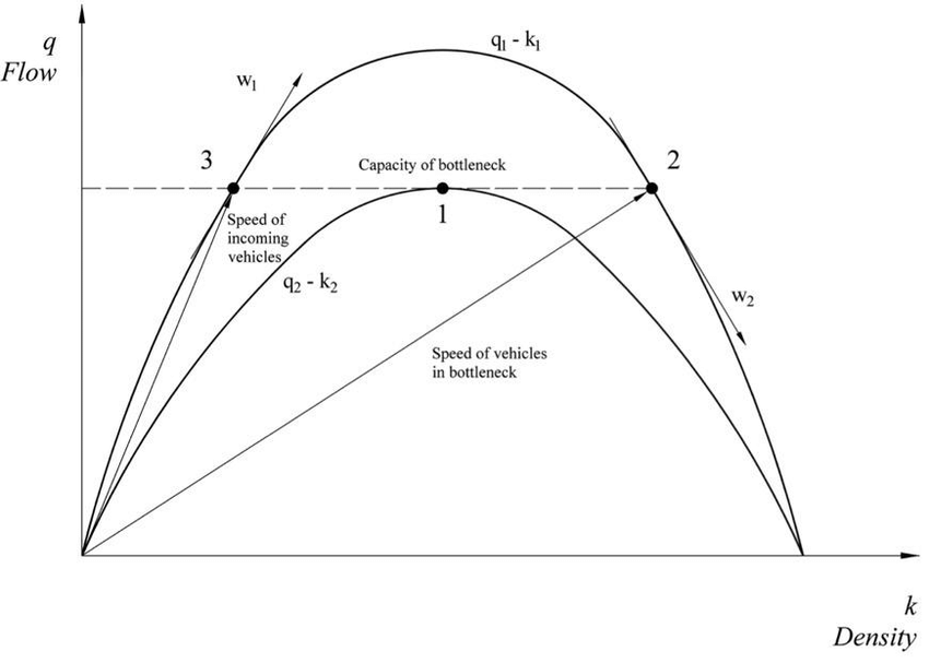
• The curve q₁-k₁ in the diagram represents the carriageway downstream of the bottleneck, and the curve q₂-k₂ refers to the bottleneck itself.
• When the traffic volume reaches the capacity of the bottleneck, denoted by number 1 in the diagram, it is clear that the velocity of the bottleneck itself is less than that downstream of the bottleneck.
• An additional increase in traffic volume accumulates as a queue upstream of the bottleneck, causing a shift of the traffic state to another (from traffic conditions at the point 3 to those at the point 2 in the diagram), i.e. density changes from k₃ to k₂ (Drew, 1968).
• Let Q_A represent the flow, which is less than Q’_m. The capacity of the bottleneck on entering the bottleneck, the concentration increases from k_A to k_B.
• The mean speed of vehicles in the road, ^QA/_KA drops down to ^QB/_KB.
• No shock wave is formed.